
Evaluating Agent Performance
Evaluation with LLMs
September 4, 2026
When the output of an LLM-based or agentic system is too open-ended to define a deterministic unit test, LLM-as-a-judge has become the go-to method to evaluate systems. The idea sounds simple: instead of writing a fixed test, you give a second AI system or LLM the system output, together with a judge prompt (detailed instructions on how to grade the output, much like a teacher's marking guide) and ask it to return a verdict such as pass/fail or a label like "good" or "bad".
This can be a very useful and powerful method to evaluate qualities that are hard to capture in deterministic rules. Think of tone of voice, whether a generated summary captures the main point, or whether a generated piece of text contradicts itself. Without thinking too much about it, this approach seems credible. If AI systems are 'smart' enough that we can ask them to do certain tasks, why not use other AI systems to check that our systems are working correctly?
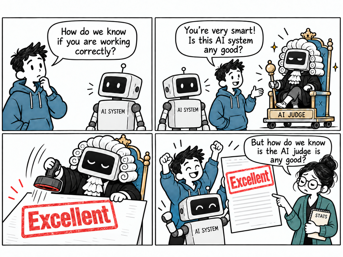
But handing the evaluation to another AI system often moves the problem rather than solving it. We wanted to know how reliable an AI system is. Having passed that question to a second AI system, we are left with the same question one level up: how reliable is the judge?
To establish the statistical reliability of the LLM-as-a-judge method, we need to carefully track a few details that are easily overlooked:
- how often the judge agrees with human experts
- how many expert-labelled examples that agreement was measured on
- how large the uncertainty on that measured agreement is
- whether the errors of different judges are correlated
- whether the judge is consistently too lenient or too strict (more on this in the next section) Only by carefully keeping track of errors, sample sizes, and corelations, can we tell whether a judge's verdicts are reliable, or are themselves mostly hallucination and statistical noise.
In the rest of this first section, we will discus the LLM-as-judge method in detail: best practices on how to establish the accuracy of this method. What to watch out for, and where the limits of this method lie. We then work through an example rubric, and show how to design evaluations that keep the LLM's role as small as possible by relying on rule-based checks wherever we can.
In later sections we show how to go beyond this, and build up towards rigurous methodologies for the governance of Agentic AI systems.
The LLM-as-a-Judge Method in More Detail
For each criterion that we want to jude the output on, a 'judge prompt' is written. This judge prompt gives the LLM criterion-specific instructions, questions and examples, ideally written in collaboration with subject matter experts (SMEs). The LLM then receives an example output to evaluate, together with the judge prompt, and is asked to follow the instructions to assign a label to the output. Much like a teacher marking an exam using a grading guideline, we ask the LLM to pick a label from a fixed set like ['excellent', 'good', 'bad', 'terrible'], or simply pass/fail
An LLM is trained to predict the next token in a piece of text. When we ask it to generate a label based on the instructions in a judge prompt, nothing guarantees that the assigned label will be correct.
One way to try to make the LLM output more reliable, is to have the LLM first generates a series of intermediate thinking steps, before it produces its final label. For some types of questions, this approach can result in more reliable answers. But it comes also with the side effect that once the LLM starts writing out its reasoning, it can quickly become convinced of its own line of argument. We will return to this, and how to optimise judge prompts, as well as how to also make use of the log probabilities in the LLM output, in later sections.
Once the judge prompts are written, we measure how well the LLM-as-a-judge implementation performs on each criterion, again usually together with SMEs. By checking the fraction of examples on which the LLM-as-a-judge implementation assigns the same label as the SME, we find the reliability of a specific criterion.
The set of SME-labelled examples has to be large enough (typically at least 100–500) for the measured reliability to mean much. We will see why in the section on sampling error below.
When a judge scores poorly on a criterion, there are several ways to improve it. We discuss these in later sections.
An Example Rubric (and how to track reliability)
To make this all more concrete, consider an example system that writes summaries based on a set of source documents. Below is a very minimal example rubric, to evaluate the quality of the resulting summaries against three example criteria. Each criteria is using LLM-as-a-judge in a different way:
-
Full LLM judge: the LLM decides the verdict on its own, based on a judge prompt. This is the most flexible approach, but also the least reliable.
-
LLM as an atomic step: the LLM performs only one narrow, well-defined task (e.g. "does this passage support this claim?") inside a chain of otherwise rule-based steps. Keeping the LLM's role small makes the metric more reliable.
-
Rule-based check: the verdict follows entirely from explicit, programmatic rules-based checks (e.g. matching section headings against a required list), with no LLM involved.
Here we deliberately avoid calling rule-based checks 'deterministic'. An LLM run at temperature 0 is sometimes also described as deterministic. Though in practice that doesn't hold exactly: floating-point rounding on GPUs and batching effects can still change the output between runs. More importantly, determinism is not what makes a metric reliable. A temperature-0 judge can give the same wrong verdict every time. What sets rule-based checks apart is that their logic is explicit: allowing us to know with a much higher reliability which cases will be handled correctly.
| # | Metric | How it is evaluated | Role of the LLM | Measured agreement with SMEs |
|---|---|---|---|---|
| 1 | Formal tone of voice | LLM-as-a-judge with SME written judge prompt: 'is the register formal?' → fail if answer is "no" | Full LLM-as-a-judge | 73.0% |
| 2 | Factual consistency | LLM extracts atomic claims from the summary → for each pair, LLM answers "Do these two claims contradict each other?" yes/ne → fail if any single pair contradicts | Aatomic steps: claim extraction and contradiction check | 82.0% |
| 3 | Required sections present | Parse the section headings with regex patterns and compare them against a fixed list of required headings → fail if any required section is missing | None (rule-based) | 100% |
In the above example, metric 2 also illustrates how errors pile up along a chain.
Suppose the claim extraction step works correctly 99.9% of the time, and the pairwise contradiction check is correct 99.5% of the time. If on average a summary contains 10 claims, it require pairwise comparisons. The chance that the whole chain results in a correct evaluation is then roughly . A step accuracy that sounds excellent (99.5%) turns into roughly 80% when we run it multiple times.
Tracking individual step accuracies is useful for finding which steps to improve. But always measure the chain end-to-end against the SMEs, rather than multiplying step accuracies when assessing the total reliability. In practice, errors in different steps can also cancel or reinforce each other.
The measured agreement rates in the above table are specific for the exact setup that was used. Means that the measured numbers in the above table holds only for
- one particular set of curated SME-annotated examples
- one specific LLM (including version number, temperature, and other inference settings)
- one particular version of the judge prompt
Change any of these, and every number has to be measured again.
How certain are we about the accuracy?
Every measured number comes with a sampling error. When we throw a six-sided die, and average the values we throw, it should average out to 3.5 when we throw an infinite number of times. But suppose we throw a die 100 times, and get an average of 3.71. Does that mean the die is unfair? Not necessarily: over only 100 throws, even a perfect die will sometimes turn up a few more sixes than expected. The 3.71 you measured has an error margin around it, and the true average will lie somewhere within that range.
Now imagine repeating this experiment many times, each time we throw the die 100 times and calculating the average. Each time we might obtain a different value: . Over many repetitions these sample averages would form a distribution centered around the true value of 3.5. The width of this distribution is the standard error on our estimate.
If instead of averaging over 100 throws, we average 1,000 throws each time. The resulting averages will generally cluster much more tightly around 3.5. A few extra ones or sixes might still appear during some runs, but they will have less influence on the final average when each estimate is averaged over ten times as many throws.
In general, the error decreases with . where is the number of observations. Increasing the sample size improves precision, but with diminishing returns: halving the error takes four times as many observations.
A judge's accuracy works the same way. If a judge agrees with the SMEs 80% of the time, we need to find out what the error margin is on that 80%.
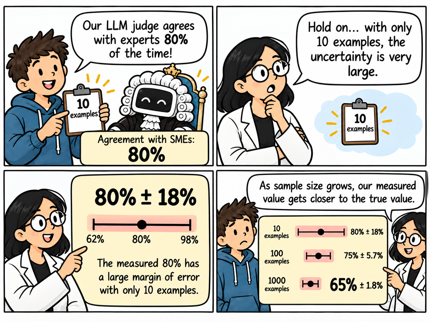
For simplicity, we treat each agreement rate as a binomial proportion measured on examples, with a standard error (all errors in this post are at 1σ).
Measuring 80% agreement on 100 examples then gives , or roughly ±8 points at 95% confidence. One hundred examples sounds rigorous, but it still leaves a wide band on the judge's true accuracy. And because the error only shrinks as , halving it takes four times as much SME labelling effort.
The binomial error breaks down close to 0% or 100%: "99.5% ± 0.5%" suggests the true value could exceed 100%. Near the edges, use a Wilson interval instead, which can be asymmetric.
Adding the 1σ errors to our rubric allows us to track how certain we are about the reliability of each metric:
| # | Metric | How it is evaluated | Role of the LLM | Measured agreement with SMEs | Number of SMEs curated examples |
|---|---|---|---|---|---|
| 1 | Formal tone of voice | LLM-as-a-judge with SME written judge prompt: 'is the vocal register formal?' → fail if answer is "no" | Full LLM-as-a-judge | 73.0% ± 13.4% | |
| 2 | Factual consistency | LLM extracts atomic claims from the summary → for each pair, LLM answers "Do these two claims contradict each other?" yes/ne → fail if any single pair contradicts | Aatomic steps: claim extraction and contradiction check | 82.0% ± 2.7% | $N = 225% |
| 3 | Required sections present | Parse the section headings with regex patterns and compare them against a fixed list of required headings → fail if any required section is missing | None (rule-based) | 100% | doesn't apply |
Combining different metrics into one score
When we make changes to our system, we rarely improve only one criterion at a time. A different system prompt might make answers follow the required format better, but also make them more verbose. Two different system prompts might impact the different criterea in our rubric differently. Making it difficult to compare both changes.
By combining the different metrics with different weights into a single combined score, we make it possible to do A/B comparisons across different model versions, by simply comparing their total scores to evaluate the performance of the system as whole. . The price of collapsing everything into one number is that the uncertainties of all the individual criteria flow into it as well.
If the final evaluation score is the weighted sum of the rubric pass rates . Then the statistical error would be (if the metrics were independent) .
When labels like "excellent/good/bad/terrible" are converted to , the final total evaluation function, as well as the variance you compute depends on an arbitrary choice of spacing. Change the spacing to and changes with it.
In practice, though, metrics are often not independent. The more criteria we add, the more likely it is that some of them are correlated. With correlations between the metrics (where ), the error becomes .
Notice how the uncertainties compound: criteria with large individual errors, and criteria whose errors are correlated, both push the error on the final score above what we would naively estimate.
This quadrature-sum addition of the errors assumes the errors behave like independent Gaussian noise. For LLM judges that is rarely the case. Their errors tend to be input-dependent: on some inputs a judge hallucinates far more than on others, as a result the errors are not randomly distributed. [2] discusses this in more detail in the context of combining multiple LLM juries into a panel, with the aim of obtaining more reliable results.
Judges on similar criteria are likely to be correlated with each other: they tend to be wrong in the same way, rather than in independent, random ways. This makes it difficult in practice to gain accuracy by simply adding more judges or more criteria. [1] discusses this in the context of combining multiple LLM judges into a panel of judges (wich is sometimes done with the aim of obtaining more reliable results).
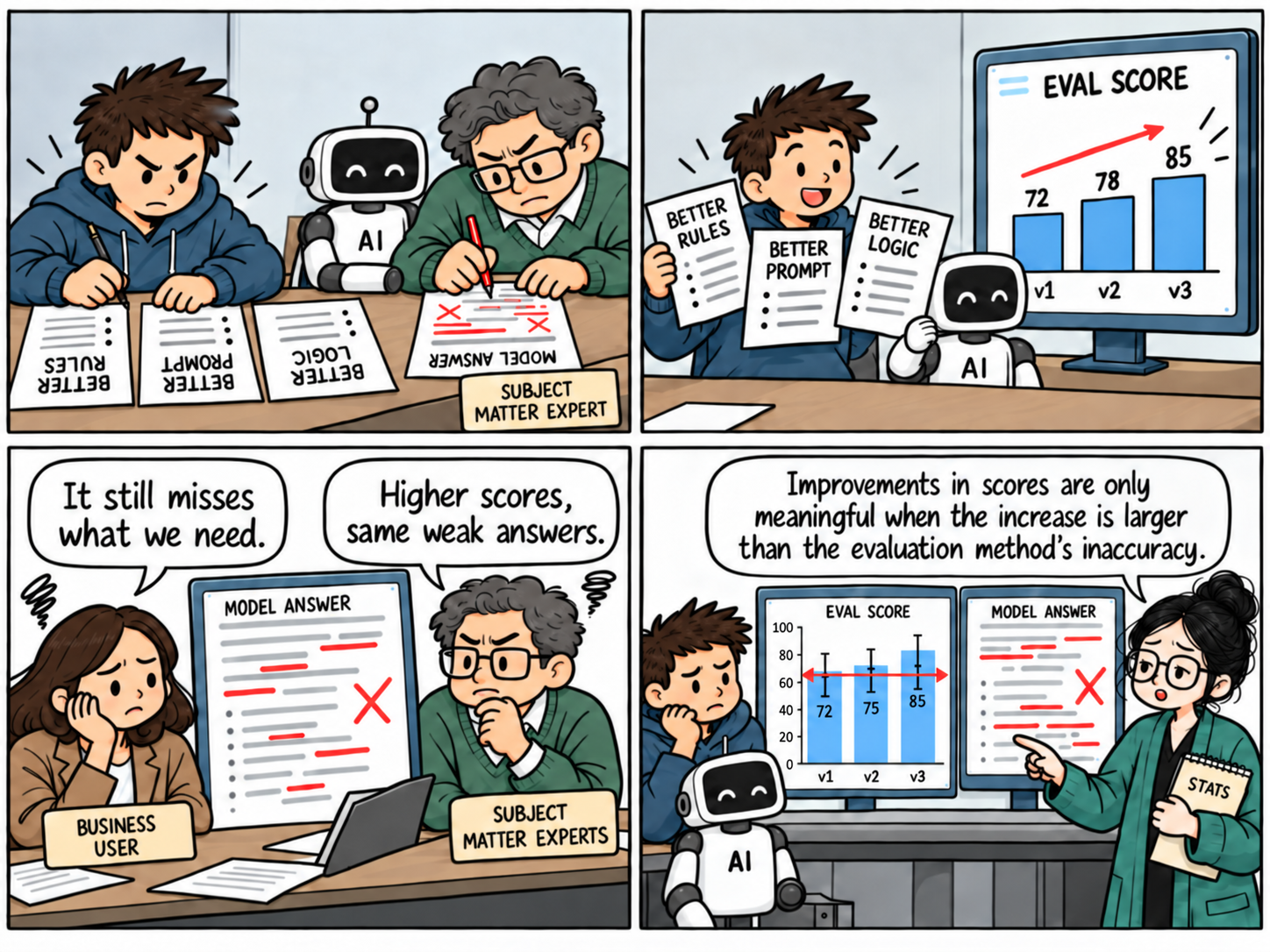
The statistical error on our evaluation metric sets the smallest improvement we can meaningfully detect.
When we compare two versions of a system (with different logic, different prompts or different LLMs), a difference in score smaller than about two standard errors of that difference may not be significant at 95% confidence. For two independent evaluations with error each, that threshold is .
Why this is important
Over the past few years I've seen methods like LLM-as-a-judge being implemented to evaluate engineering projects at more and more companies. Under tight delivery deadlines, this often looks like a quick win. LLM-as-a-judge often gives the impression that it we have verified in a quantifiable way that a system does what it is supposed to do. This is especially appealing for chatbots and other LLM-based systems, performing loosely defined functions, for which it can be difficult to evaluate the performance using deterministic acceptance tests.
But projects that lean too heavily on hastily implemented LLM-as-a-judge evaluations often get stuck. Without carefully tracking the reliability of the judge systems, teams end up running round in circles. They tweak system prompts, and update parts of their application logic, attempting to push up their own evaluation scores, only to hear users and SMEs say that, despire the higher evaluation scores, the output hasn't really improved. Steering towards genuine improvement becomes difficult, for one main reason: without knowing how accurate the judges are, there is no way to tell whether a higher score reflects better performance or just statistical noise.
A related approach, sometimes known as Council of LLMs, combines multiple LLM Judges into a panel to improve their accuracy. This is usually justified with a handwaving 'wisdom of the crowds' argument; combining many small, individual judgments into one final answer, allows to average out errors and extreme guesses, causing the average to converge to the truth
Lately, as LLM-as-a-judge becomes increasingly popular. Particularly on vibe coded projects, there is also growing pile of quickly produced documentation on how to set it up, and with it a growing body of folk wisdoms surrounding the topic. Statements like:
- make sure to let the LLM generates labels as output.
- convert the labels to numbers if you want to combine them.
- and make sure you don't use the same LLM to judge as system as the one that is running the system. To prevent any bias confirmation.
These statements sound reasonable enough, until you start asking quantitative questions about them:
- How repeatable is a label generated by an LLM judge? How likely is it to produce the wrong label?
- How does the choice of the numerical scale, when mapping labels to numbers influence the final score, and the accuracy in our final score.
- What counts as a 'different' LLM exactly? Is a different model version of the same LLM from the same company already different enough? Or should it have a completely different architecture? Or should it have been trained on a different dataset?
The folk wisdom can't answer these quantitative questions. But careful measurements, and statistics can. This is what the rest of this series sets out to do.